Brazilian Pricing Models¶

This is a technical description of Everysk's Brazilian pricing models, organized in 6 sections:

Description of underlying risk factors
Pricing formulas for local fixed income, futures, and derivatives
Formulas for sensitivities required in the risk models
Formulas for parametric risk measures
Formulas and examples for stress tests
Liquidity measures

SECTION 1: RISK FACTORS¶

The first step of the process is the decomposition of each security into its underlying risk factors in order to compute how these factors interact with each other.

Risk factors that can be reliably utilized for forecasting need to be independent and identically distributed (i.i.d.). For example: non-overlapping compounded returns rather than closing prices should be used as the risk factor for a stock. In what follows we describe why:

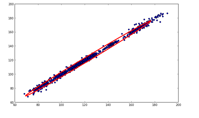
The scatterplot below shows the daily closing prices of a stock in the x-axis with the 1-day lagged prices in the y-axis. In red, we plot the location-dispersion ellipsoid to represent the covariance between the samples. It can be seen that there is a very uneven amount of variance projected to the principal axis of the ellipsoid. The series of closing prices cannot be considered independent.

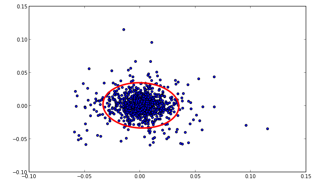
Conversely, the 1-day lagged scatterplot of non-overlapping compounded returns is shown below. The corresponding location-dispersion ellipsoid is almost a circle, indicating that compounded returns are independently distributed and can be used as a risk factor in forecasting. Whereas compound returns are used for stocks (lognormal), absolute variations in level are used as risk factors for rates and credit spreads (normal)

Primitive risk factors used by Everysk include:

Constant Maturity DI1xPRE: We store on a daily basis the following key rate duration points in the DI1xPRE curve (basis 252 days): 1 month, 6months, 1 year, 5 years, 10 years, 30 years
Constant Maturity DI1xDOL: We store on a daily basis the following key rate duration points in the DI1xDOL curve (basis 252 days): 1 month, 6months, 1 year, 5 years, 10 years, 30 years
Constant Maturity Ibovespa: We store on a daily basis the following forward points in the IBOV future curve: 1 month, 6months, 1 year, 5 years, 10 years, 30 years
Constant Maturity BRLUSD: We store on a daily basis the following forward points in the BRLUSD curve: 1 month, 6months, 1 year, 5 years, 10 years, 30 years
Constant Maturity DIxIPCA: We store on a daily basis the following forward points in the DIxIPCA curve: 1 month, 6months, 1 year, 5 years, 10 years, 30 years

Similar to other practitioners we use an exponentially weighted moving average (EWMA) of squared returns (or absolute level variations) as as an estimate of volatility for the primitive risk factors. For example: if we observe daily returns from time t-k to time t, we can describe the one-day volatility estimate as :

\[ \sigma = \large \left[\frac{1-\lambda}{1-\lambda^{k+1}}\right] \sum_{i=0}^{k} \lambda^{i} \ r_{t-i}^{2}\]

The $\lambda$ parameter is designed to put more emphasis on more recent data and will be described below. When we assume two risk factors, the above formula takes into account the correlation:

\[ \Sigma_{ij} = \large \left[\frac{1-\lambda}{1-\lambda^{k+1}}\right] \sum_{i=0}^{k} \lambda^{i} \ r_{t-i}^{j} \ r_{t-i}^{j}\]

Here we have substituted the squared returns by the product between returns from each asset. If the assets move in the same direction, the 2 assets amplify their risk when together in a portfolio. If the assets move in opposite directions, they buffer risk. The formula above is effectively the same as:

\[\Sigma_{ij} = \large \rho_{ij} \ \sigma_{i} \ \sigma_{j} \]

The covariance matrix is just an assembly of all the cross-volatilities and correlations from the above formula.

The optimal level of decay ($\lambda$) in the formulas above is found by minimizing the mean squared errors between the forecasted volatility (variance) and the actual realized squared returns each day. Practitioners have found that 0.94 is a good estimate for daily volatility and 0.97 for monthly. Using a 0.94 decay puts 90% of the weight in the last 38 days of historical returns (log(0.10)/log(0.94)).

SECTION2: PRICING FORMULAS¶

Before we describe the portfolio risk statistics in part 3, we need to provide a mapping between risk factors and pricing formulas. We start with pricing formulas for publicly issued fixed income:

NTN-B:¶

This is an inflation-linked bond issued by the National Treasury with a face value of R$1000 that pays semi-annual coupons of 6%, with inflation correction by the IPCA index (Broad consumer price index, published by IBGE):

\[ \large \text{PU} = \sum_{i=1}^{n} \frac{\text{\small{IPCA}}_{total} \times \text{VNE} \times \left[(1.06)^{0.5}-1\right]}{(1+ytm)^{\frac{DU_{i}}{252}}} + \frac{\text{\small{IPCA}}_{total} \times \text{VNE} }{(1+ytm)^{\frac{DU_{T}}{252}}}\]

where:

PU: unit price
VNE: Face value at issuance - R$1000
ytm: yield that is found by equating the present value of cashflows to the PU
DU: business days between pricing date and event date (coupon, amortization, maturity)
$\text{\small{IPCA}}_{total}$ is the inflation adjustment that depends on the date that the bond is being priced as follows:

1) Bond being priced on a date falling between the last published IPCA and the 15th of the month:

\[\text{\small{IPCA}}_{total} = \large \frac{\text{IPCA}_{t-1}}{\text{IPCA}_{0}} \ \times \left[\frac{\text{IPCA}_{t-1}}{\text{IPCA}_{t-2}}\right]^{\frac{DU_{1}}{DU_{2}}} \]

where $\text{IPCA}_{0}$ is the value of the index prevailing in the month prior to the bond issuance and $\text{IPCA}_{t-1}$ is the value of the index prevailing on the month prior to the calculation date and $\text{IPCA}_{t-2}$ is the value prevailing 2 months prior to calculation date. $DU_{1} / DU_{2}$ is the pro-rata number of days between last and current 15th of the month.

2) Bond being priced on the 15th of the month:

\[\text{\small{IPCA}}_{total} = \large \frac{\text{IPCA}_{t}}{\text{IPCA}_{0}}\]

where $\text{IPCA}_{0}$ is the value of the index prevailing in the month prior to the bond issuance and $\text{IPCA}_{t}$ is the value of the index prevailing on the calculation date (15th).

3) Bond being priced on a date falling between the 15th of the month and next IPCA to be published

\[\text{\small{IPCA}}_{total} = \large \frac{\text{IPCA}_{t-1}}{\text{IPCA}_{0}} \ \times \left[1+\text{IPCA}_{proj}\right]^{\frac{DU_{1}}{DU_{2}}}\]

where $\text{IPCA}_{0}$ is the value of the index prevailing in the month prior to the bond issuance and $\text{IPCA}_{t-1}$ is the value of the index prevailing prior to the calculation date and $\text{IPCA}_{proj}$ is the projected IPCA, published by ANBIMA. $DU_{1} / DU_{2}$ is the pro-rata number of days between last and current 15th of the month.

| - Internal symbology: BRRF:NTNB_YYYYMMDD PU | BRRF:NTNB_20350515 4153.0872 - Display symbology: NTNB_20350515 | | --- |

NTN-C:¶

This is an inflation-linked bond issued by the National Treasury with a face value of R$1000 that pays semi-annual coupons of 12%, with inflation correction by the IGP-M index (market price index, published by Fundaçāo Getulio Vargas):

\[ \text{PU} = \large \sum_{i=1}^{n} \frac{\text{\small{IGPM}}_{total} \times \text{VNE} \times \left[(1.12)^{0.5}-1\right]}{(1+ytm)^{\frac{DU_{i}}{252}}} + \frac{\text{\small{IGPM}}_{total} \times \text{VNE} }{(1+ytm)^{\frac{DU_{T}}{252}}}\]

where $\text{\small{IGPM}}_{total}$ is calculated depending on the date that the bond is being priced, as follows:

1) Bond being priced on a date falling between the last published IGP-M and the 1st of the month:

\[\text{\small{IGPM}}_{total} = \large \frac{\text{IGPM}_{t-1}}{\text{IGPM}_{0}} \ \times \left[\frac{\text{IGPM}_{t}}{\text{IGPM}_{t-1}}\right]^{\frac{DU_{1}}{DU_{2}}} \]

where $\text{IGPM}_{0}$ is the value of the index prevailing in the month prior to the bond issuance and $\text{IGPM}_{t-1}$ is the value of the index prevailing on the month prior to the calculation date and $\text{IGPM}_{t}$ is the value prevailing on the calculation date. $DU_{1}$ represents the number of days between the first of the month to calculation date and $DU_{2}$ is the number of days between the first day of the last month and current 1st of the month.

2) Bond being priced on the 1st of the month:

\[\text{\small{IGPM}}_{total} = \large \frac{\text{IGPM}_{t}}{\text{IGPM}_{0}}\]

3) Bond being priced on a date falling between the 1st of the month and next IGP-M to be published

\[\text{\small{IPCA}}_{total} = \large \frac{\text{IGPM}_{t-1}}{\text{IGPM}_{0}} \ \times \left[1+\text{IGPM}_{proj}\right]^{\frac{DU_{1}}{DU_{2}}}\]

where $\text{IGPM}_{0}$ is the value of the index prevailing in the month prior to the bond issuance and $\text{IGPM}_{t-1}$ is the value of the index prevailing on the prior month and $\text{IGPM}_{proj}$ is the value of the index forecasted by ANBIMA. $DU_{1}$ represents the number of days from the first day of prior month and calculation date. $DU_{2}$ is number of days between current and next 1st of the month.

| - Internal symbology: BRRF:NTNC_YYYYMMDD PU | BRRF:NTNC_20210401 4932.1647 - Display symbology: NTNC_20210401 | | --- |

NTN-F:¶

This is an nominal bond issued by the National Treasury with a face value of R$1000 that pays semi-annual coupons of 10%:

\[ \text{PU} = \large \sum_{i=1}^{n} \frac{ \text{VNE} \times \left[(1.10)^{0.5}-1\right]}{(1+ytm)^{\frac{DU_{i}}{252}}} + \frac{ \text{VNE} }{(1+ytm)^{\frac{DU_{T}}{252}}}\]

where:

PU: unit price
VNE: Face value at issuance - R$1000
ytm: yield that is found by equating the present value of cashflows to the PU
DU: business days between pricing date and event date (coupon, amortization, maturity)

| - Internal symbology: BRRF:NTNF_YYYYMMDD PU | BRRF:NTNF_20310101 1177.6526 - Display symbology: NTNF_20310101 | | --- |

LTN:¶

This is a zero coupon bond issued by the National Treasury with face value of R$1000.

\[ \text{PU} = \large \frac{ \text{VNE} }{(1+ytm)^{\frac{DU_{T}}{252}}}\]

where:

PU: unit price
VNE: Face value at issuance - R$1000
ytm: yield that is found by equating the present value of payout at maturity to the PU
$DU_{T}$: business days between pricing date and maturity

| - Internal symbology: BRRF:LTN_YYYYMMDD PU | BRRF:LTN_20240101 822.1798 - Display symbology: LTN_20240101 | | --- |

LFT¶

This is a zero coupon floating bond issued by the National Treasury with face value of R$1000.

\[\text{PU} = \large \frac{ \text{VNE} \ \times \prod_{i=1}^{DU} \left[ (1+selic_{i})^{\frac{1}{252}}-1\right]}{(1+ytm)^{\frac{DU_{T}}{252}}}\]

where:

PU: unit price
VNE: Face value at issuance - R$1000
ytm: yield that is found by equating the present value of payout at maturity to the PU
$DU_{T}$: business days between pricing date and maturity
selic: 100% of the inter bank rate accrued from issuance to calculation date

| - Internal symbology: BRRF:LFT_YYYYMMDD PU | BRRF:LFT_20240901 10586.1295 - Display symbology: LFT_20240901 | | --- |

And privately issued fixed income:

Formulas below assume the most generic case of amortizing principal:

\[ \text{\small{VNA}}_{i} = \large \text{\small{VNE}} \times \left[1- \sum_{t=0}^{i-1} \small{\text{Amort}}_{t}\right] \]

where $\text{Amort}_{i}$ are principal amortizations as percent of VNE. The initial VNA for calculating the bonds below, takes into account all the amortizations that occurred from issuance to the pricing date.

Debentures paying percent of DI (interbank deposit rates):¶

These debentures pay a percent (pct) of projected DI. The forwards are built using forward DI contracts at specific vertices.

\[ \text{PU} = \large \sum_{i=1}^{n} \frac{\text{\small{VNA}}_{i-1} \times \text{cpn}_{i} + \left[\text{\small{VNA}}_{i-1} - \text{\small{VNA}}_{i}\right] }{(1+ytm)^{\frac{DU_{i}}{252}}}\]

where:

For first coupon

\[ \text{cpn}_{1} = \large \left[\prod_{i=1}^{n} \left[1+\left[(1+\text{\small{DI1}}_{i})^{\frac{1}{252}} -1 \right] \times pct \right] \right]\times \left[ 1+\left[(1+fwd_{1})^{\frac{1}{252}}-1\right]\times pct\right]^{DU_{1}} \]

where DI1 is accrued from issuance to calculation date, and remaining coupons:

\[ \text{cpn}_{2 \dots n} = \large \frac{\left[ 1+\left[(1+fwd_{i})^{\frac{1}{252}}-1\right]\times pct\right]^{DU_{i}}}{\left[ 1+\left[(1+fwd_{i-1})^{\frac{1}{252}}-1\right]\times pct\right]^{DU_{i-1}}}\]

| - Internal symbology: BRRF:TICKER PU | BRRF:CEEBA2 10114.25 - Display symbology: CEEBA2 | | --- |

Debentures paying DI + spread:¶

These debentures pay a spread over projected DI. The forwards are built using forward DI contracts at specific vertices.

\[\text{PU} = \large \sum_{i=1}^{n} \frac{\text{\small{VNA}}_{i-1} \times \text{cpn}_{i} + \left[\text{\small{VNA}}_{i-1} - \text{\small{VNA}}_{i}\right] }{(1+ytm)^{\frac{DU_{i}}{252}}}\]

For first coupon:

\[ \text{cpn}_{1} = \large \left[\prod_{i=1}^{n} (1+\text{\small{DI1}}_{i})^{\frac{1}{252}}\right]\times (1+\text{spread})^{\frac{{DU}_{1}}{252}}\]

For remaining coupons:

\[ \text{cpn}_{2 \dots n} = \large (1+\text{spread})^{\frac{{DU}_{i}}{252}}\]

| - Internal symbology: BRRF:TICKER PU | BRRF:ENGIA2 1009.63 - Display symbology: ENGIA2 | | --- |

Debentures paying IPCA + spread:¶

These bonds pay a coupon and principal amortizations that are inflation adjusted with IPCA:

\[\text{PU} = \large \sum_{i=1}^{n} \frac{\text{\small{IPCA}}_{total} \times \left[\left[\text{VNA}_{i-1} \ \times (1+ \text{spread})^{\frac{DU_{i}}{252}}\right] + \left[\text{VNA}_{i-1} - \text{VNA}_{i-1}\right]\right]}{(1+ytm)^{\frac{DU_{i}}{252}}} \]

where $\text{\small{IPCA}}_{total}$ is computed similarly than NTN-B above.

| - Internal symbology: BRRF:TICKER PU | BRRF:AGRU41 1236.31 - Display symbology: AGRU41 | | --- |

CRA paying DI + spread:¶

Pricing is very similar to debentures paying DI + spread. The only difference here is that because this is a securitized bond, it contains an offset for coupon payment that affects the first coupon as follows:

\[\text{cpn}_{1} = \large \left[\prod_{i=\text{def}}^{n} (1+\text{\small{DI1}}_{i})^{\frac{1}{252}}\right]\times \left[(1+fwd_{1})^{\frac{(DU_{1}-\text{def})}{252}}\ \times(1+\text{spread})^{\frac{{DU}_{1}}{252}}\right]\]

where $\bold{def}$ is the offset in days defined in the terms of the securitization.

| - Internal symbology: BRRF:ISIN PU | BRRF:CRA019007Q8 1048.4344 - Display symbology: CRA019007Q8 | | --- |

CRA paying percent of DI:¶

Pricing is very similar to debentures paying a percent of DI. The only difference here is that because this is a securitized bond, it contains an offset for coupon payment that affects the first coupon as follows:

\[ \text{cpn}_{1} = \large \left[\prod_{i=\bold{\text{def}}}^{n} \left[1+\left[(1+\text{\small{DI1}}_{i})^{\frac{1}{252}} -1 \right] \times pct \right] \right]\times \left[ 1+\left[(1+fwd_{1})^{\frac{1}{252}}-1\right]\times pct\right]^{(DU_{1}-\text{def})}\]

where $\bold{def}$ is the offset in days defined in the terms of the securitization.

DI1 Futures:¶

This cash settled future pays the capitalized daily Interbank Deposit (DI) rates verified on the period between the trading day, including, and the last trading day, including.

It's PU is:

\[\text{PU} = \large \frac{ \text{100000} }{(1+\text{rate})^{\frac{DU_{T}}{252}}}\]

where:

PU: unit price
rate: quoted rate
$DU_{T}$: business days between pricing date and expiration of the contract

The multiplier for the contract is BRL 1.00

| - Internal symbology: BRFUT:DI1 YYYYMMDD PU | BRFUT:DI1 20210104 99442.31 - Display symbology: DI1J21 | | --- |

DDI Futures:¶

This cash settled future pays the difference between the capitalized daily Interbank Deposit (DI) rates and the FX variation verified on the period between the trading day, including, and the last trading day, including.

It's PU is:

\[\text{PU} = \large \frac{ \text{100000} }{(1+\text{CC} \times \frac{DC_{T}}{360})}\]

where:

PU: unit price
CC: quoted "coupon cambial"
$DC_{T}$: running days between pricing date and expiration of the contract

and:

\[\text{CC} = \left[\frac{ \text{PTAX}_{T} }{\text{PTAX}_{0}} \times {(1+\text{rate})^{\frac{DU_{T}}{252}}} - 1 \right] \times \frac{360}{DC_{T}}\]

$\text{PTAX}_{0}$: spot exchange rate of Brazilian reais for US dollars, offer side, as quoted by the Brazilian Central Bank (Bacen)
$\text{PTAX}_{T}$: forward exchange rate of Brazilian reais for US dollars as per FX futures contract
rate: daily Interbank Deposit (DI) rates as per DI1 futures

The multiplier for the contract is USD 0.50

| - Internal symbology: BRFUT:IDI YYYYMMDD PU | BRFUT:IDI 20210915 100267.8 - Display symbology: DDIU21 | | --- |

IND / WIN Futures:¶

These cash settled futures pay the price appreciation/depreciation of the Ibovespa index. The only difference between the contracts are the multipliers: BRL 1.00 for IND and BRL 0.20 for the WIN contract.

| - Internal symbology: BRFUT:WIN YYYYMMDD PU | BRFUT:WIN 20201014 20038.55 - Display symbology: WINZ20 | | --- |

ISP / WSP Futures:¶

These cash settled futures pay the price appreciation/depreciation of the SP500 index in Reais. The only difference between the contracts are the multipliers: USD 50.00 for ISP and USD 2.50 for the WSP contract.

| - Internal symbology: BRFUT:ISP YYYYMMDD PU| BRFUT:ISP 20210315 3319.25 - Display symbology: ISPM21 | | --- |

DOL / WDO Futures:¶

These cash settled futures pay the difference between a USD settlement at a pre-agreed rate and the FX at expiration. The contract size is USD 50,000 and the mini contract, WDO, controls USD 10,000

\[\large \text{PU}_t = \text{PTAX}_{t-1} \times \frac{\text{PU}_{ddi}}{\text{PU}_{di1}} = \text{PTAX}_{t-1} \times \frac{(1+\text{rate})^{\frac{DU_{T}}{252}}}{(1+\text{CC} \times \frac{DC_{T}}{360})}\]

| - Internal symbology: BRFUT:DOL YYYYMMDD PU | BRFUT:DOL 20210315 5646.45 - Display symbology: DOLM21 | | --- |

DAP Futures:¶

These cash settled futures pay the spread between the compounded DI rate, in the period between the calculation date, including, and the expiration date, excluding, and the IPCA variation verified in the period as of the calculation date until and including the expiration date. It compensates buyers from inflation erosion, paying a real interest rate.

\[\large \text{PU} = \frac{\text{100000}}{(1+\text{spread}_{\small{\text{DI1xIPCA}}})^{\frac{DU_{T}}{252}}}\]

| - Internal symbology: BRFUT:DAP YYYYMMDD PU| BRFUT:DAP 20220815 25.45 - Display symbology: DAPQ22 | | --- |

The multiplier for this contract is BRL 0.00025.

Stock options:¶

Stock options are priced with the Black and Scholes equation:

\[ \large \text{PU} = \psi \ S \ \Phi (\psi \ d_1) - \psi \ K * e^{-r(\text{T}-t)} * \Phi (\psi [ d_1 - \sigma \sqrt{\text{T}-t}])\]

where

\[ \large d_1 = \frac{ln(S/K)+(r+0.5\overline{\sigma}^2)(T-t)}{\sigma\sqrt{\text{T}-t}}\]

and: $\Phi$ is cumulative function for a normal distribution and $\psi$ is an indicator function equal to one for calls and -1 for puts

| - Internal symbology: BBDC4:BVMF YYYYMMDD STRIKE PREMIUM (see here) - Example: BBDC4:BVMF 20200921 C22.12 0.017735 - Display symbology: BBDCI267 | | --- |

IDI options:¶

IDI options are priced with the Black 76 equation:

\[\large \text{PU} = (1 + \text{DI1})^{-\frac{\text{DU}}{252}} \left[ \psi \ F \ \Phi (\psi \ d_1) - \psi \ K \Phi (\psi [ d_1 - \sigma \sqrt{\text{T}-t}]\right]\]

\[ \large d_1 = \frac{ln(F/K)+(r+0.5\overline{\sigma}^2)(T-t)}{\sigma\sqrt{\text{T}-t}}\]

And the forward is:

\[ \large F = \text{IDI}_{t} \times (1 + \text{DI1})^{\frac{\text{DU}}{252}} \]

where: $\text{IDI}_{t}$ is the spot DI index published by CETIP, $\Phi$ is the cumulative function for a normal distribution and $\psi$ is an indicator function equal to one for calls and -1 for puts

| - Internal symbology: BROPT:IDI YYYYMMDD STRIKE PREMIUM (see here) - Example: BROPT:IDI 20210104 P287900 632.06 - Display symbology: IDIFPG2 | | --- |

Other pricing formulas including offshore instruments can be found in our white paper. More symbology examples can be found in symbology.

SECTION 3: SENSITIVITY MEASURES¶

We compute various sensitivity measures that are needed for parametric VaR and stress tests, namely:

MACAULAY DURATION:¶

\[ \text{Macaulay Duration} = \large \frac{\sum_{i=1}^{n} \ ({\text{CF}_{i} }/{DF_{i}}) \times DU_{i}}{Price} \]

$\bold{CF}$ are the periodic bond cashflows, described in the previous chapter. $\bold{DF}$ are the discount factors used to present value cashflows. For example, for the NTN-B bond, the calculation of duration in fractional years:

\[\frac{\left[\sum_{i=1}^{n} \frac{\text{\small{IPCA}}_{total} \times \text{VNE} \times \left[(1.06)^{0.5}-1\right]}{(1+ytm)^{\frac{DU_{i}}{252}}} \times \text{DU}_{i} \right] + \left[\frac{\text{\small{IPCA}}_{total} \times \text{VNE} }{(1+ytm)^{\frac{DU_{T}}{252}}} \times \text{DU}_{T}\right]}{(\text{PU} \times 252)}\]

MODIFIED DURATION:¶

\[\text{Modified Duration} = \large \frac{\small{\text{Macaulay Duration}}}{(1+\frac{\text{ytm}}{n})}\]

where:

n is the number of cashflows
ytm is the yield to maturity of the bond

EFFECTIVE DURATION:¶

\[ \text{Effective Duration} = \large \frac{\text{P}_{-\Delta \text{yield}}-\text{P}_{+\Delta \text{yield}}}{2\text{P}\Delta_{\text{yield}}}\]

where the shift in yield, $\Delta_{\text{yield}}$ is +-1% for calculations. For a NTN-F, the formula for PU becomes:

\[\text{PU}_{\Delta} = \large \sum_{i=1}^{n} \frac{ \text{VNE} \times \left[(1.10)^{0.5}-1\right]}{(1+ytm+\Delta)^{\frac{DU_{i}}{252}}} + \frac{ \text{VNE} }{(1+ytm+\Delta)^{\frac{DU_{T}}{252}}}\]

CONVEXITY:¶

\[ \text{Convexity} = \large \frac{\text{P}_{-\Delta \text{yield}}- 2 \text{P} + \text{P}_{+\Delta \text{yield}}}{\overline{\Delta_{\text{yield}}}^{2}} \]

SECTION 4: RISK MEASURES¶

¶

PARAMETRIC VAR¶

The calculation of parametric VaR requires a measure of potential P&L distribution. Let's start describing how the profit and loss (P&L) of a single security changes with changes in risk factors. For illustration purposes, lets assume that the security depends on a single risk factor:

\[ \text{P\&L} = \large \frac{\partial P}{\partial \text{f}} \ \Delta \text{f}\]

where $\frac{\partial P}{\partial \text{f}}$ is the sensitivity of price $\bold{P}$ to changes in the risk factor $\bold{f}$. If a security depends on multiple risk factors:

\[ \text{P\&L} = \large \sum_{i=0}^{n}\frac{\partial P}{\partial \text{f}_{i}} \ \Delta \text{f}_{i} \]

Or in matrix format:

\[ \text{P\&L} = \large \widetilde{P}^{T} \ \ \widetilde{f} \]

The equation above can be stated as the internal product of a vector of sensitivities (delta equivalents) and primitive risk factor returns. The portfolio P&L is obtained by simply adding the individual security P&Ls.

FROM P&L DISTRIBUTION TO VaR

The main objective of a parametric approach to VaR is to generate a distribution of P&L without the need of simulations and then infer statistical properties from the distribution. Because primitive risk factors are normally distributed and any linear combination of a normal distribution preserves normality (parametric model linearizes the relationship between risk factors and price variation), a reasonable P&L distribution can be drawn from the following normal distribution:

\[ \text{P\&L} \sim \large N(0 \ , \ \widetilde{P}^{T} \ \Sigma \ \widetilde{P}) \]

To calculate VaR using the parametric approach, we simply note that VaR is always a multiple of the standard deviation for a normal distribution:

\[ \text{VaR} = \large -1.64 \times \sqrt{\widetilde{P}^{T} \ \Sigma \ \widetilde{P}} \times \sqrt{T} \]

The above equation measures the "T" horizon value at risk with 95% confidence (1.64 is the 95% percentile)

Let's work an example from beginning to end, demonstrating how the parametric VaR is calculated. Assume we hold BRL 1M worth of PETR4 stock and BRL 1M face value of NTN-B, expiring on may 2035. The NTN-B has a price of R$ 4316 and the Petrobras stock R$ 23.41. This 2-asset portfolio would contain 3 risk factors, namely: Petrobras returns, 10 year and 30 year constant maturity synthetic durations.

The vector of total portfolio sensitivities, $\widetilde{P}$, would be (columns are assets and rows are primitive risk factors):

	PETR4	NTN-B 2035	$\widetilde{P}$
PETR4	R$ 1,000,000	0	R$ 1,000,000
10 year DIxPRE	0	-R$ 9,739,747	-R$ 9,739,747
30 year DIxPRE	0	-R$ 779,980	-R$ 779,980

(*)Everysk allows primitive risk factors for stocks to be the stock return or an Index, via Betas.The stock entry is trivial, the sensitivity of Petrobras stock to itself is 1, therefore the entry in the sensitivity matrix is just: 42717 shares x R$23.41/share x 1 (sensitivity). The entries for the NTN-B in the sensitivity matrix are a bit more complex. We need to find a blend between a 10 year and 30 year durations, given the duration of the NTN-B.

Assume the duration of the bond in years is $\small D$, falling between 2 key rates durations, $\small T_1$ and $\small T_2$. The linear interpolation is calculated as $\alpha * \text{rate}_{T1} +(1-\alpha) * \text{rate}_{T2}$. If the duration of the NTN-B is 10.5 years:

\[ \alpha = \frac{(T_2-D)}{(T_2-T_1)} = \frac{(30.0-10.5)}{(30.0-10.0)} = 97.5\%\]

We will map 97.5% of the $1M NTN-B to a synthetic 10 year constant maturity bond and 2.5% to a 30 year. The entries in the sensitivity matrix are:

-R$ 9,739,747 = 232(quantity) * R$ 4316 (unit price) * 10 (sensitivity) * 97.5% (blend mapping) and
-R$ 779,980 = 232(quantity) * R$ 4316 (unit price) * 30 (sensitivity) * 2.5% (blend mapping).

The negative signs indicate that the price of the bond is inversely related to rates. If the absolute level of rates contract, the bond appreciates.

Those individual sensitivities are joined via the covariance of primitive risk factors, $\Sigma$. Using the returns (percent or absolute) and EWMA decay, the covariance for risk factors would be (all numbers are x 10-6):

	PETR4	10 year DIxPRE	30 year DIxPRE
PETR4	61	-33	-31
10 year DIxPRE	-33	4	3.2
30 year DIxPRE	-31	3.2	4.2

Finally the VaR (daily, 95% confidence) can be calculated with simple matrix operations:$$\text{VaR} = \large -1.64 \times \sqrt{\widetilde{P}^{T} \ \Sigma \ \widetilde{P}}$$where $\widetilde{P}^{T}$ is the transpose of total portfolio sensitivity vector:$$\widetilde{P} = \left[ \begin{array}{cccc} R$ \ 1,000,000 \ -R$ \ 9,739,747 \ -R$ \ 779,980 \end{array}\right] $$The result of the calculation above is a VaR of -R$ 56,402. To calculate the VaR in percentage terms we simply divide the result by the net asset value of the portfolio, R$2M, resulting in $\bold{-2.82\%}$. That means that a portfolio comprised 50/50 of Petrobras stock and NTN-B may 2035 would have 5% of probability of losing 2.82% or more in a day.

INCREMENTAL VAR - IVAR¶

Another important measure for portfolio risk management is Incremental VaR. IVAR measures the changes in portfolio VaR to changes in the portfolio holdings. The parametric formula is:$$\text{IVaR} = \large -1.64 \times \frac{\widetilde{P} .* \Sigma \ \widetilde{P}}{\sqrt{\widetilde{P}^{T} \ \Sigma \ \widetilde{P}}}$$where the numerator of the ratio above is an element-wise vector multiplication. A desirable property of incremental VaR is that it adds to total portfolio risk. If we substitute the values for our illustrative portfolio with Petrobras and NTN-B:

$$ \text{IVaR} = \left[ \begin{array}{cccc} -R$ \ 19,388.51 && -R$ \ 34,580.23 && -R$ \ 2,434.07\end{array}\right] $$ The last 2 entries represent the NTN-B. Thus the contribution to VaR as percent of the portfolio is:

$$ \text{IVaR} = \left[ \begin{array}{cccc} -R$ \ 19,388.51 && -R$ \ 37,014.30\end{array}\right] / R$ \ 2\text{M} = \left[ \begin{array}{cccc} -0.97\% && -1.85\%\end{array}\right]$$ As it can be seen above, the incremental VaR for Petrobras (-0.97%) plus NTN-B (-1.85%) adds to total portfolio VaR of -2.82%.4.3) EXPECTED SHORTFALL

A complementary measure to VaR is Conditional VaR (also called expected shortfall).Expected Shortfall is a risk statistic that describes how large losses are on average when they exceed the VaR level. Re-writing the equation for P&L below:

\[ \text{P\&L} = \large \widetilde{P}^{T} \ \ \widetilde{f} \]

If $\widetilde{P}^{T}$ is a vector with dimensions $1 \times m$, where m is the number of primitive risk factors. $\widetilde{f}$ is a matrix of dimensions $m \times n$ with risk factor returns where the rows are factors and columns are historical dates going back $\bold{n}$ days.

The resulting vector of $\bold{n}$ P&Ls can then be ordered from lowest to highest. Then, the average of the worst 5% P&Ls (95% confidence) will be the expected shortfall. Mathematically it is defined as:
$$ \large \text{E}\left[\text{-P\&L} \ | \ \text{-P\&L}>\text{VaR}\right]$$or:$$\text{CVaR} = -\left[\text{VaR} \ + \frac{1}{(1-\alpha)\text{n}} \times \sum_{i=1}^{\text{n}} \text{max}(\text{P\&L}_{i}-\text{VaR},0)\right]$$Where $\alpha$ is the confidence level (95%). In the illustrative example with one NTN-B and one Petrobras stock the expected shortfall is -6.15%, a much larger potential loss than the VaR. Expected shortfall measures the "tail risk" of the P&L distribution. The contribution to tail risk from each security in the portfolio can be easily retrieved by using the same sort from the overall portfolio and averaging the worst X-percentile security P&Ls. $$\large \text{P\&L}{i} = \large \widetilde{P} $$}^{T} \ \ \widetilde{fSECTION 5: STRESS TESTSThe risk measures above are complemented by stress tests. Parametric stress tests are computed similarly to above measures, with the difference that the primitive factor returns are exogenously provided as extreme shocks.Back to our illustrative example of a portfolio comprised of 2 assets: a Petrobras stock and a NTN-B, we could ask ourselves what is the expected P&L of the portfolio in a flight to quality represented by the Bovespa index down 10% and rates contracting 100bps (parallel move in the curve):The new sensitivity matrix now uses the Bovespa as a risk factor, which is connected to the Petrobras stock via Petrobras beta of 1.26 in the example:

	PETR4	NTN-B 2035	$\widetilde{P}$
IBOV	R$ 1,260,000	0	R$ 1,260,000
10 year DIxPRE	0	-R$ 9,739,747	-R$ 9,739,747
30 year DIxPRE	0	-R$ 779,980	-R$ 779,980

Thus:$$ \text{PL}{st} = \left[ \begin{array}{cccc} R$ \ 1,260,000 && -R$ \ 9,739,747 && -R$ \ 779,980\end{array}\right] \times\left[ \begin{array}{cccc} -0.1 \ -0.01 \ -0.01\end{array}\right] $$$$ \text{PL} = = -R$ \ 20,802.73$$In terms of percent of net liquidating value (R$ 2M), the shocked P&L above equates to a loss of -1.04% (most of the P&L loss from Petrobras is compensated by an appreciation from the NTN-B.Beyond user-defined shock vectors like above, Everysk also calculates B3 and CVM (regulatory) stress tests.

B3 SHOCK MATRIX¶

B3 publishes a matrix of prescribed shocks. For interest rate (DIxPRE) and coupon shocks, it provides shocks for 3 vertices, namely: 6 months, 1 year and 5 years. For each vertex, it publishes a low and high shock projected ahead for 1 day, 5 days and 10 days.

Current Pre-DI curve shocks (all in %):

	Low	High
6 months	-1.20	-1.60
1 year	-1.40	-1.85
5 years	-1.90	-2.60

(*) 3 values per cell, indicating a 1 day | 5 day | 10 day horizons.

The duration of the bond is used to interpolate/extrapolate shocks provided in the 0.5,1,5 year vertices.

Current coupon cambial shocks (all in %):

	Low	High
6 months	-1.75	-1.95
1 year	-1.55	-1.80
5 years	-1.25	-1.70

(*) 3 values per cell, indicating a 1 day | 5 day | 10 day horizons.

Current BRLUSD shocks (all in %)

	Low	High
NA	-12.00	-14.10

Current Ibovespa shocks (all in %):

	Low	High
NA	-18.00	-28.20

Let's use our illustrative portfolio of R$1M NTN-B 2035 expiring in May and R$1M of Petrobras stock. If we are interested on the worst P&L for a 5 day horizon, we would perform 16 stress tests as follows:

For each position:

First collect the low/high shocks for 5 days: Because the duration of the NTN-B is 10.5 years, it extrapolates a 10 year and 30 year shocks from the 5 year - in our implementation it simply extends the same B3 shocks beyond 5 years:

(-2.60, +3.70),(-2.60, +3.70),(-1.70, +2.85),(-1.70, +2.85),(-14.10, +19.60),(-28.20, +25.20)

Were the tuples above represent 5-day horizon low/high shocks for: 10 year duration DIxPRE, 30 year duration DIxPRE, 10 year coupon, 30 year coupon, FX and Ibovespa.

Then we compute the cartesian product of all these tuples, generating 64 combinations (in a real example the combinations are much higher):

(-2.60,-2.60, -1.70, -1.70, -14.10, -28.20), (-2.60,-2.60, -1.70, -1.70, -14.10, +25.20), ...

Finally we compute the P&L resulting from the internal product of portfolio sensitivities and each combination above:

\[ \begin{array}{ccc} \text{PL}_{st} = \left[-R\$ 9,739,747 \ | -R\$ 779,980 \ | R\$ \ 0 \ | R\$ \ 0 \ | R\$ \ 0 \ |R\$ \ 1,260,000\right] \times \\ \\ \\ \\\left[ \begin{array}{cccc} -0.026 && -0.026 && \dots \\ -0.026 && -0.026&& \dots\\ -0.017&& -0.017&& \dots\\ -0.017&& -0.017&& \dots\\ -0.141&& -0.141&& \dots\\ -0.282&& +0.252&& \dots\end{array}\right]\end{array}\]

where the first matrix of dimensions $1 \times 6$ are the sensitivities to 10 year rates, 30 year rates, 10 year coupon, 30 year coupon, FX and Ibovespa in that order. The second matrix with dimensions $6 \times 64$ represent all the combinations of B3 shocks.

The matrix multiplication results on a vector of P&Ls that can expressed as a percentage of portfolio NAV:

\[\text{PL}_{st} = \left[-4.09\% , \ +29.55\% , \ \dots\right]\]

The largest negative P&L is used as the final result. Certain combinations that might generate large negative P&Ls might have low probability to occur.

HISTORICAL STRESS TESTS¶

Historical stress tests are designed to probe adverse historical market events in order to model how the current portfolio might withstand similar situations in the future. For example: in general when risky assets like the Ibovespa index decline, there is a flight to quality and rates contract (prices of fixed income assets go up).

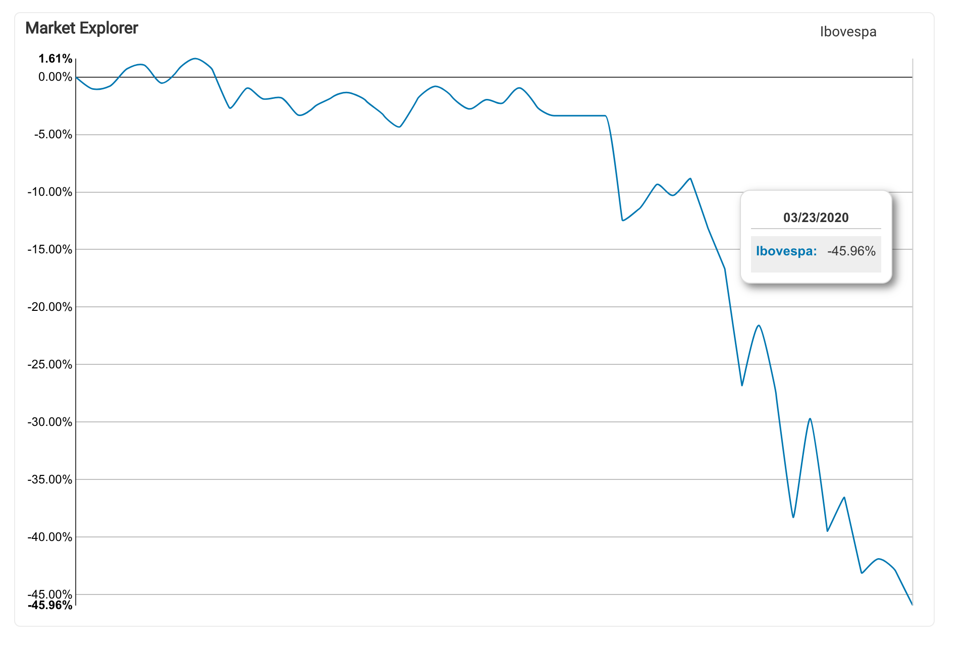
Therefore, rates spreads and the index are positively correlated. Sometimes though, this correlation breaks: more recently in mid-January 2020 the IBovespa declined 45% and instead of experiencing a contraction, the 10 year constant maturity point of the curve widened. Bonds and the index both declined, offering no diversification when together in a portfolio:

From mid January to mid March 2020, the IBovespa experienced a 46% decline:

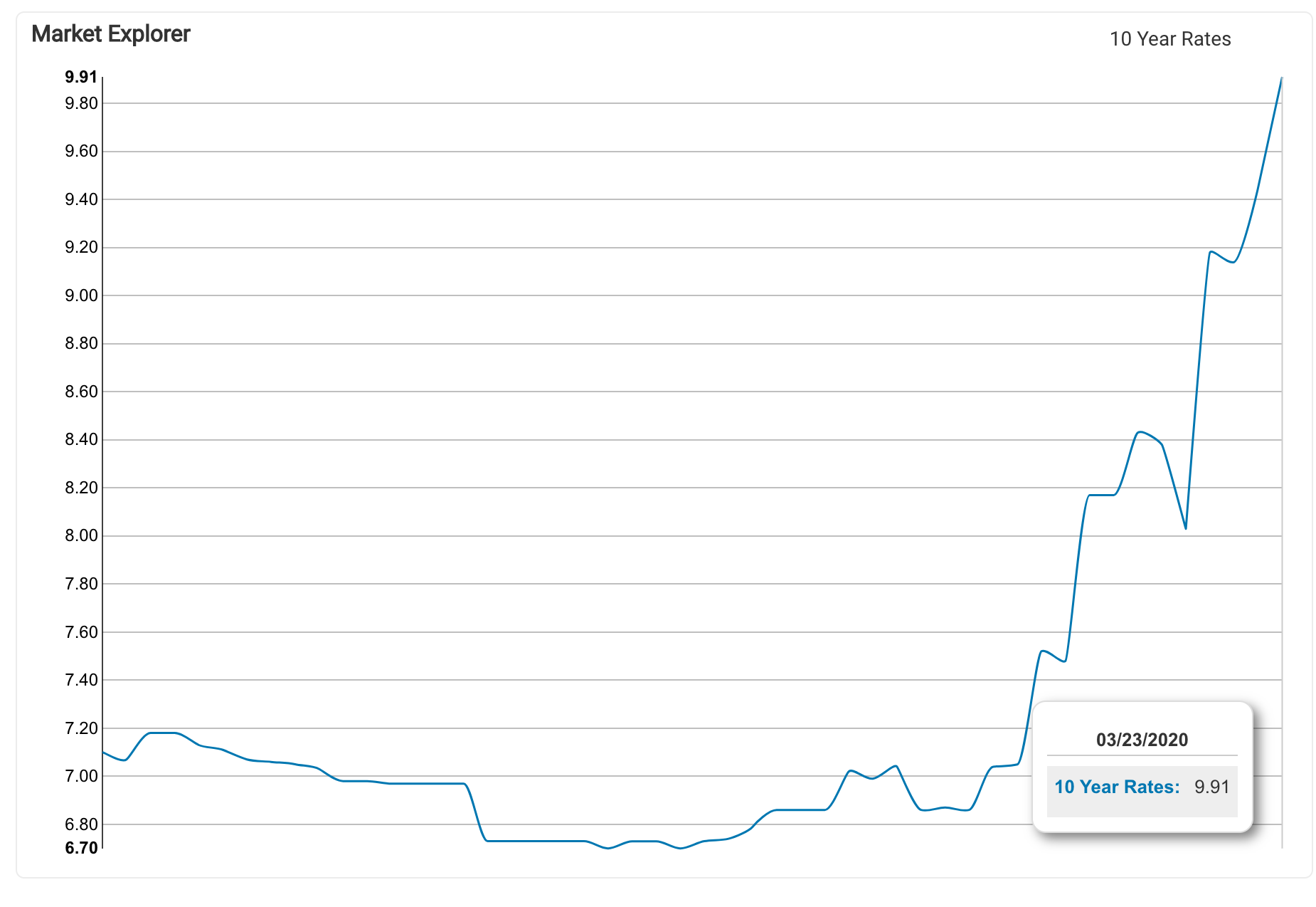
During the same period, the 10 year rates widened almost 300 basis points, from 7.10% to 9.91%:

This historical scenario above would be very detrimental to our illustrative portfolio with NTN-B and Petrobras, as follows:

$$ \text{PL}{st} = \left[ \begin{array}{cccc} R$ \ 1,260,000 && -R$ \ 9,739,747 && -R$ \ 779,980\end{array}\right] \times\left[ \begin{array}{cccc} -0.4596 \ 0.0281 \ 0.0273\end{array}\right] $$$$ \text{PL} = = -R$ \ 874,076.34$$. For a portfolio with a $2M net asset value, this represents a 43% decline in value.

When evaluating the effect of historical stress tests that span a period of many months (or years), users should be careful when drawing direct comparisons with a B3 shock, projected from 1 to 10 days.

SECTION 6: LIQUIDITY¶

ASSET LIQUIDITY:

Everysk calculates what percentage of portfolio can be unwound at various user-defined liquidity vertices. The process has two steps. namely: 1) the days to unwind (DTU) is calculated for each security; and 2) the market value of the security is bucketed on the closest liquidity vertex greater or equal than the DTU:

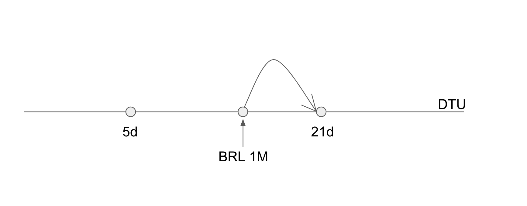
For example: In the schematic above it takes 15 days to unwind (see formulas below) a security with BRL 1M in market value. That amount would be bucketed in the next liquidity vertex, 21 days.

DTU Calculations:¶

Equity¶

The days to unwind is calculated as:

\[ \text{DTU} = \large \frac{\text{quantity}}{\text{participation} \times \text{ADTV}} \]

where:

quantity is the number of shares held in the portfolio
ADTV is the average daily trading volume computed in a window of X-days, where X can be specified by user and defaults to 20 days.
participation is a percent of total volume assumed to be available to unwind the position in full. Can be specified by user and defaults to 20%

Public Bonds¶

The days to unwind is calculated as:

\[ \text{DTU} = \large \frac{\text{quantity}}{\text{participation} \times \text{ADTV}} \]

where:

quantity is the number of bonds held in the portfolio
ADTV is the average daily trading volume computed in a window of X-days, where X can be specified by user and defaults to 20 days. ADTV published by Brazilian Central Bank on a daily basis
participation is a percent of total volume assumed to be available to unwind the position in full. Can be specified by user and defaults to 10%

Debentures¶

Liquidity for debentures is based on traded volume. If a debenture hardly trades (definition of threshold below), then Everysk uses cashflow events and reduces the amount paid by the reductions published by ANBIMA:

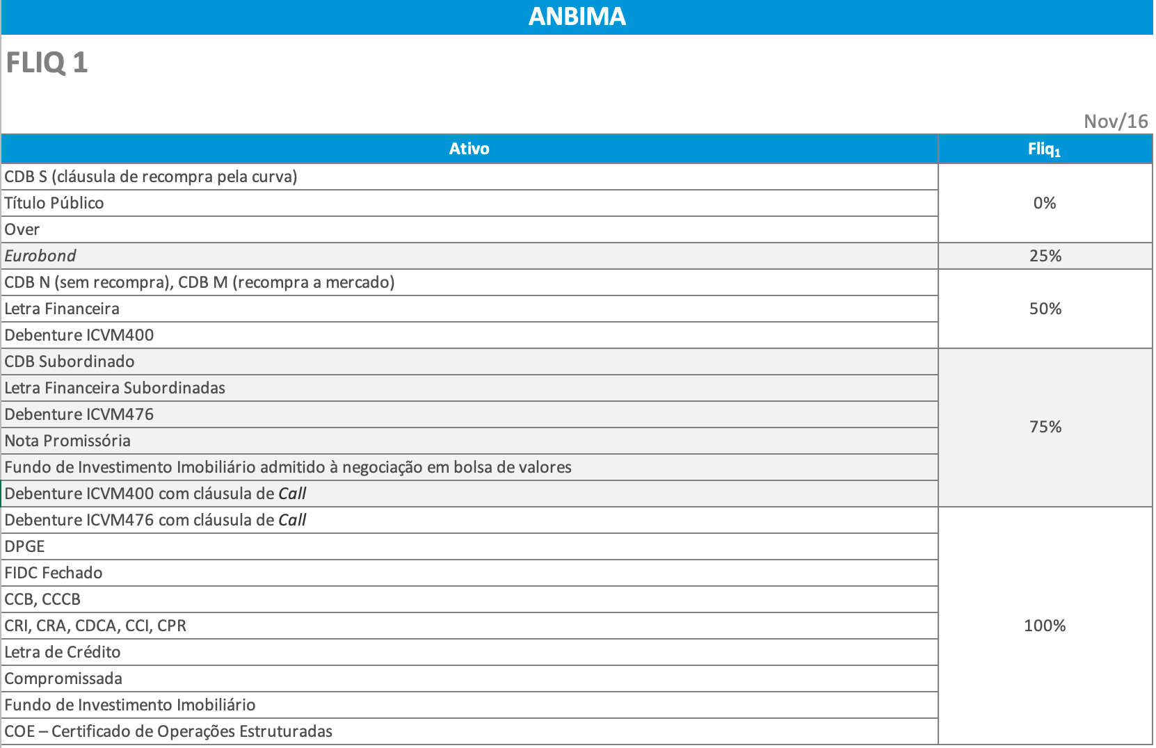
For liquid debentures (at least 20 bonds traded on a 20 day window, i.e. averaging one trade a day), Everysk uses the average volume information instead of a liquidity reduction:

\[ \text{DTU} = \large \frac{\text{quantity}}{\text{participation} \times \text{ADTV}} \]

FLIQ1 = FLIQ2 = 0%

For illiquid debentures (less than 20 bonds traded on a 20 day window, i.e. averaging less than one trade a day), Everysk uses the maturity in fractional years times 252 days:

\[ \text{DTU} = \large \text{DU}_{T} \times 252 \]

And the amount of cash generated is multiplied by the liquidity reduction

\[\large \text{CF}_{T} \times (1-\text{FLIQ1}) \times (1-\text{FLIQ2})\]

Except for some Debentures (currently around 60) that have FLIQ2=50%, all others are considered with FLIQ2=0%

Funds¶

Supplied by user as a lookup between the fund CNPJ (EIN) and days to unwind

Mapping to a liquidity vertex:

Assume that a position of $1M in a security can be unwound in 6.8 days (DTU=6.8 calculated as per above) and the vertices are 1,5,21,42,63,126, 252 and 252+ days. Further assume that the portfolio has $2M net asset value, the row corresponding to this security in the liquidity vector would be:

1d	5d	21d	42d	63d	126d	252d	252+
0%	0%	50%	50%	50%	50%	50%	50%

Thus, 50% of portfolio can be unwound in 21 days or longer, which is the nearest vertex greater or equal to 6.8 days. If the other $1M was represented by an illiquid debenture, with maturity in 5 years, the total liquidity matrix would be:

	1d	5d	21d	42d	63d	126d	252d	252+
liquid	0%	0%	50%	50%	50%	50%	50%	50%
illiquid	0%	0%	0%	0%	0%	0%	0%	25%
Total	0%	0%	50%	50%	50%	50%	50%	75%

The 25% for the illiquid asset takes into account the liquidity reduction of 50% for FLIQ1 and 0% for FLIQ2 as follows:

\[ \frac{\text{CF}_{i} \times (1-\text{FLIQ1}) \times (1-\text{FLIQ2})}{\text{NAV}} = \frac{\$ 1\text{M} \times (1-0.5) \times (1- 0.0)}{\$2\text{M}} = 25\%\]

LIABILITY PROJECTIONS:

On the liability side we use historical redemption statistics to compute daily net redemptions (redemption minus contribution) as a percent of the portfolio's net asset value - NAV ("Patrimonio Liquido") of the fund from prior date:

\[ \text{Net Redemption}_{i} = \large \frac{\text{redemptions}_{i}-\text{subscriptions}_{i}}{\text{NAV}_{i-1}}\]

Then, we compute various averages going back: 5 days, 21 days and the other vertices we used in the asset side liquidity:

\[ \text{ANRV}_{5d} = \large \frac{1}{5} \ \times \sum_{i=today-5}^{today}\frac{\text{redemptions}_{i}-\text{subscriptions}_{i}}{\text{NAV}_{i-1}}\]

Finally the values that are used in the vertices are the cumulative sums of average redemptions to that point, so the redemption at the 21 days includes all the redemptions as a percent of NAV for 5 days and 21 days and so forth.

ASSET-LIABILITY COVERAGE:

Once we have calculated the liquidity in the portfolio at various vertices (1d,5d,21d,...) and redemption forecasts in the same vertices, we can compute the asset-liability coverage on each vertex:

\[\large \text{Coverage}_{5d} = \large \text{Liquidity}_{5d}-\text{Projected Redemptions}_{5d}\]