Debt-Equity trades
Background
Debt-equity trades are hard to analyze. Traditionally it is not trivial to hedge out the common factors driving both credit and equity.
In general buy-side firms have sophisticated models to analyze the sensitivity of each leg of the trade separately, but they lack a robust way to propagate common risks. For example, how a trade involving a CDS and a put option might behave due to movements in the underlying stock? The put option would be trivial: the trader might have a volatility surface to compute various option prices for different underlying prices. But the CDS is more complex: how changes in stock price propagate to spreads and probabilities of default? Simple regressions of stocks and credit spreads will yield incorrect results.
This is where Everysk can complement buy-side models by simulating the cross-asset propagation, so that the trader or risk manager can stress-test her/his trade assumptions.
In what follows we will illustrate how it is done. Let's use an illustrative capital structure arbitrage trade involving Macy’s with 2 OTC legs: a short 5year Macy’s credit and short put option:
- CDS:M 20230924 P1.5204
- M 20200118 P32 3.81
The 2 legs above follow our symbology: the first is a 5 year credit default swap on Macy’s with 2023 maturity and paying 152.04 bps spread over Libor (short credit). The second leg is a put option on Macy’s expiring on January 2020 struck at 32 dollars and with a mid-price of 3.81 dollars.
The notional for the 5yr payor CDS is 1M dollars and the trade is setup short 300 put contracts. Additionally we are assuming that the portfolio equity is 1M dollars. Presumably this trade was established by the client with a jump-to-default scenario in mind, who now wants to stress-test its behavior within a holding period. The plots below simulate a 6 months holding period and a wide range of stock shocks: [-40% , +40%].
Starting with the put option by itself:
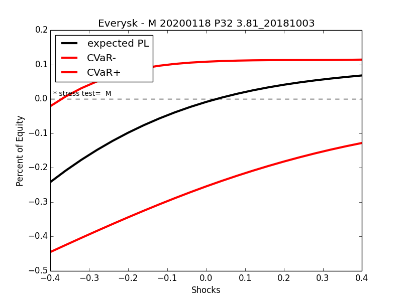
The x-axis are shocks in Macy's stock, ranging from -40% to +40%. The y-axis plots the expected profit and loss (PL) in black and 2 envelopes with the best and worst 5-percentile PLs in red.
This plot contains a lot more information than simply applying shocks to the stock and repricing the put option. In that case, we would obtain a single PL for each shock that would be comparable to the black line. Everysk will produce the full dispersion around that expectation. It can be seen that for a +40% move in Macy's stock, the expectation is asymptotically converging to the best 5-percentile, which reflects the trade making a positive PL equivalent to the full premium received from the short put (gain of approximately 11%), For a -40% move, the expectation is converging to the intrinsic value of the option.
Then, looking at the CDS independently:
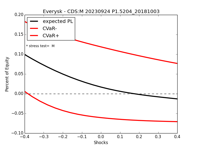
In the plot above Everysk is propagating shocks on Macy's stock to the CDS via a structural model. Additionally the negative convexity (positive for a payor swap) is captured as shown above. The expected PL for a -40% move in the stock (expected PL of +10%) is much higher than the expected loss from a symmetrical 40% up move in the stock (expected PL of -1%), due to a higher probability of default in the down move. The following table shows the calculations for various stock prices:
| Stock price ($) | Mkt Cap ($M) | Firm Value ($M) | PD | spread (%)/L |
|---|---|---|---|---|
| 95.75 | 29,394 | 34,226 | 0.46% | 0.05 |
| 46.76 (+40%) | 9.39% | 1.21 | ||
| 33.4 | 10,252 | 15,788 | 11.76% | 1.52 |
| 20.04 (-40%) | 34.88% | 5.86 | ||
| 10.90 | 3,347 | 8,179 | 50.69% | 8.87 |
The central row reflects current conditions whereas the upper and bottom rows reflect the conditions for extreme simulated stock prices. Calculations use a level of total debt of 5.5 Bi dollars, a stock volatility of 40%, an implied firm volatility of 28% and a 40% recovery value.
Finally putting both legs together:
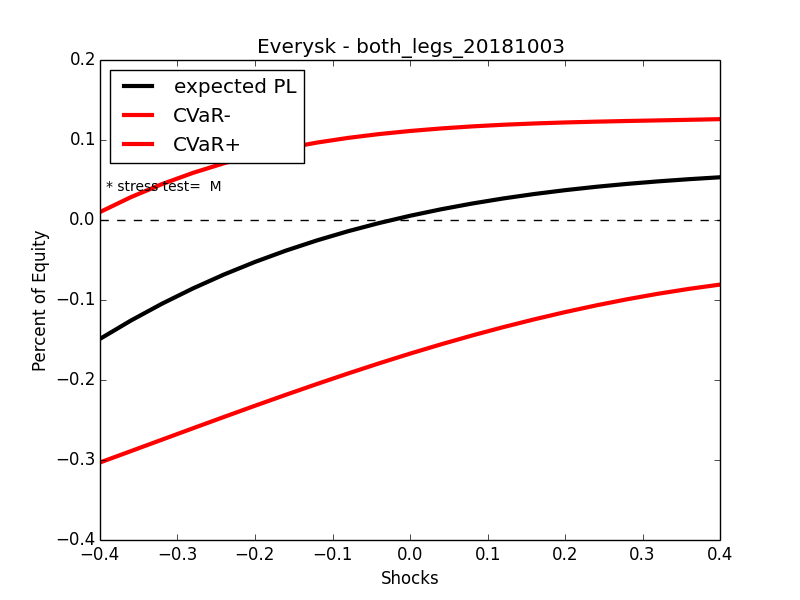
The trade might experience significant PL dispersion for a 6month horizon, despite being properly dimensioned for jump-to-default.
Other configurations that are more balanced for a 6 month horizon can be easily calculated via our API, by varying each leg quantity.
Conclusion
Everysk's transitive risk engine can be effectively used to stress test complex multi-asset trades by propagating shocks (Macy's stock in the example above) , regardless if the shock is directly used in the securities pricing or not.